The Renderers¶

General¶

Reproduction Setups¶

The geometry of the actual reproduction setup is specified in .asd files, just like sound scenes. By default, it is loaded from the file /usr/local/share/ssr/default_setup.asd. Use the --setup command line option to load another reproduction setup file. Note that the loudspeaker setups have to be convex. This is not checked by the SSR. The loudspeakers appear at the outputs of your sound card in the same order as they are specified in the .asd file, starting with channel 1.

A sample reproduction setup description:

<?xml version="1.0"?>
<asdf version="0.1">
  <header>
    <name>Circular Loudspeaker Array</name>
  </header>
  <reproduction_setup>
    <circular_array number="56">
      <first>
        <position x="1.5" y="0"/>
        <orientation azimuth="-180"/>
      </first>
    </circular_array>
  </reproduction_setup>
</asdf>

We provide the following setups in the directory data/reproduction_setups/:

2.0.asd: standard stereo setup at 1.5 mtrs distance
2.1.asd: standard stereo setup at 1.5 mtrs distance plus subwoofer
5.1.asd: standard 5.1 setup on circle with a diameter of 3 mtrs
rounded_rectangle.asd: Demonstrates how to combine circular arcs and linear array segments.
circle.asd: This is a circular array of 3 mtrs diameter composed of 56 loudspeakers.
loudspeaker_setup_with_nearly_all_features.asd: This setup describes all supported options, open it with your favorite text editor and have a look inside.

There is some limited freedom in assigning channels to loudspeakers: If you insert the element <skip number="5"/>, the specified number of output channels are skipped and the following loudspeakers get higher channel numbers accordingly.

Of course, the binaural and BRS renderers do not load a loudspeaker setup. By default, they assume the listener to reside in the coordinate origin looking straight forward.

A Note on the Timing of the Audio Signals¶

The WFS renderer is the only renderer in which the timing of the audio signals is somewhat peculiar. None of the other renderers imposes any algorithmic delay on individual source signals. Of course, if you use a renderer that is convolution based such as the BRS renderer, the employed HRIRs do alter the timing of the signals due to their inherent properties.

This is different with the WFS renderer. Here, also the propagation duration of sound from the position of the virtual source to the loudspeaker array is taken into account. This means that the farther a virtual source is located, the longer is the delay imposed on its input signal. This also holds true for plane waves: Theoretically, plane waves do originate from infinity. Though, the SSR does consider the origin point of the plane wave that is specified in ASDF. This origin point also specifies the location of the symbol that represents the respective plane wave in the GUI.

We are aware that this procedure can cause confusion and reduces the ability of a given scene of translating well between different types of renderers. In the upcoming version 0.4 of the SSR we will implement an option that will allow you specifying for each individual source whether the propagation duration of sound shall be considered by a renderer or not.

Subwoofers¶

All loudspeaker-based renderers support the use of subwoofers. Outputs of the SSR that are assigned to subwoofers receive a signal having full bandwidth. So, you will have to make sure yourself that your system lowpasses these signals appropriately before they are emitted by the subwoofers.

You might need to adjust the level of your subwoofer(s) depending on the renderers that you are using as the overall radiated power of the normal speakers cannot be predicted easily so that we cannot adjust for it automatically. For example, no matter of how many loudspeakers your setup is composed of the VBAP renderer will only use two loudspeakers at a time to present a given virtual sound source. The WFS renderer on the other hand might use 10 or 20 loudspeakers, which can clearly lead to a different sound pressure level at a given receiver location.

For convenience, ASDF allows for specifying permantent weight for loudspeakers and subwoofers using the weight attribute:

<loudspeaker model="subwoofer" weight="0.5">
  <position x="0" y="0"/>
  <orientation azimuth="0"/>
</loudspeaker>

weight is a linear factor that is always applied to the signal of this speaker. Above example will obviously attenuate the signal by approx. 6 dB. You can use two ASDF description for the same reproduction setup that differ only with respect to the subwoofer weights if you’re using different renderers on the same loudspeaker system.

Distance Attenuation¶

Note that in all renderers – except for the BRS and generic renderers –, the distance attenuation in the virtual space is \(\frac{1}{r}\) with respect to the distance \(r\) of the respective virtual point source to the reference position. Point sources closer than 0.5 m to the reference position do not experience any increase of amplitude. Virtual plane waves do not experience any algorithmic distance attenuation in any renderer.

You can specify your own preferred distance attenuation exponent \(exp\) (in \(\frac{1}{r^{exp}}\)) either via the command line argument --decay-exponent=VALUE or the configuration option DECAY_EXPONENT (see the file data/ssr.conf.example). The higher the exponent, the faster is the amplitude decay over distance. The default exponent is \(exp = 1\) [1]. Fig. 3.1 illustrates the effect of different choices of the exponent. In simple words, the smaller the exponent the slower is the amplitude decay over distance. Note that the default decay of \(\frac{1}{r}\) is theoretically correct only for infinitessimally small sound sources. Spatially extended sources, like most real world sources, exhibit a slower decay. So you might want to choose the exponent to be somewhere between 0.5 and 1. You can completely suppress any sort of distance attenuation by setting the decay exponent to 0.

The amplitude reference distance, i.e. the distance from the reference at which plane waves are as loud as the other source types (like point sources), can be set in the SSR configuration file (Section Configuration File). The desired amplitude reference distance for a given sound scene can be specified in the scene description (Section ASDF). The default value is 3 m.

The overall amplitude normalization is such that plane waves always exhibit the same amplitude independent of what amplitude reference distance and what decay exponent have been chosen. Consequently, also virtual point source always exhibit the same amplitude at amplitude reference distance, whatever it has been set to.

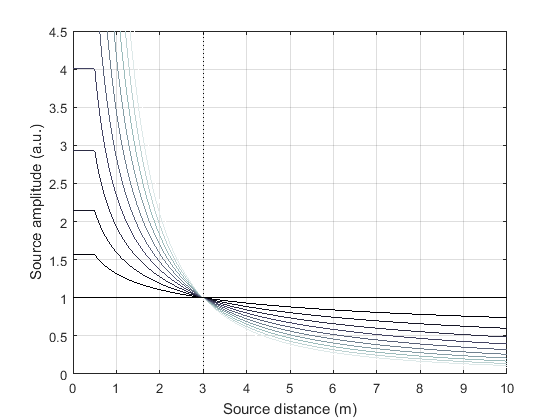
Illustration of the amplitude of virtual point sources as a function of source distance from the reference point for different exponents \(exp\). The exponents range from 0 to 2 (black color to gray color). The amplitude reference distance is set to 3 m. Recall that sources closer than 0.5 m to the reference position do not experience any further increase of amplitude.

[1]

A note regarding previous versions of the WFS renderer: In the present SSR version, the amplitude decay is handled centrally and equally for all renderers that take distance attenuation into account (see Table 2). Previously, the WFS renderer relied on the distance attenuation that was inherent to the WFS driving function. This amplitude decay is very similar to an exponent of 0.5 (instead of the current default exponent of 1.0). So you might want to set the decay exponent to 0.5 in WFS to make your scenes sound like they used to do previously.

Doppler Effect¶

In the current version of the SSR the Doppler Effect in moving sources is not supported by any of the renderers.

Signal Processing¶

All rendering algorithms are implemented on a frame-wise basis with an internal precision of 32 bit floating point. The signal processing is illustrated in Fig. 3.2.

The input signal is divided into individual frames of size nframes, whereby nframes is the frame size with which JACK is running. Then e.g. frame number \(n+1\) is processed both with previous rendering parameters \(n\) as well as with current parameters \(n+1\). It is then crossfaded between both processed frames with cosine-shaped slopes. In other words the effective frame size of the signal processing is \(2\cdot\)nframes with 50% overlap. Due to the fade-in of the frame processed with the current parameters \(n+1\), the algorithmic latency is slightly higher than for processing done with frames purely of size nframes and no crossfade.

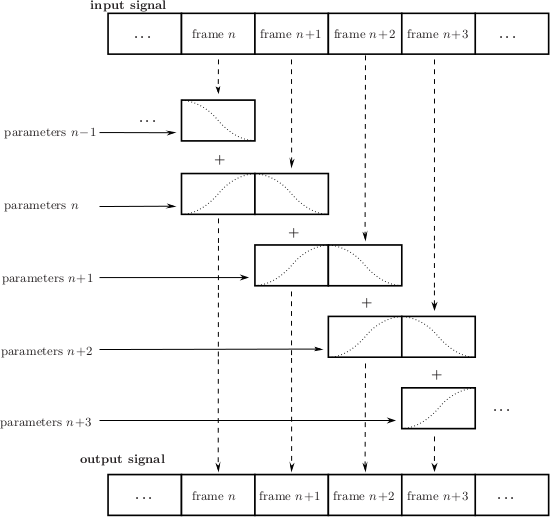
Illustration of the frame-wise signal processing as implemented in the SSR renderers (see text)

The implementation approach described above is one version of the standard way of implementing time-varying audio processing. Note however that this means that with all renderers, moving sources are not physically correctly reproduced. The physically correct reproduction of moving virtual sources as in [Ahrens2008a] and [Ahrens2008b] requires a different implementation approach which is computationally significantly more costly.

[Ahrens2008a]

Jens Ahrens and Sascha Spors. Reproduction of moving virtual sound sources with special attention to the doppler effect. In 124th Convention of the AES, Amsterdam, The Netherlands, May 17–20, 2008.

[Ahrens2008b]

Jens Ahrens and Sascha Spors. Reproduction of virtual sound sources moving at supersonic speeds in Wave Field Synthesis. In 125th Convention of the AES, San Francisco, CA, Oct. 2–5, 2008.

Binaural Renderer¶

Executable: ssr-binaural

Binaural rendering is an approach where the acoustical influence of the human head is electronically simulated to position virtual sound sources in space. Be sure that you are using headphones to listen.

The acoustical influence of the human head is coded in so-called head-related impulse responses (HRIRs) or equivalently by head-related transfer functions. The HRIRs are loaded from the file /usr/local/share/ssr/default_hrirs.wav. If you want to use different HRIRs then use the --hrirs=FILE command line option or the SSR configuration file (Section Configuration File) to specify your custom location. The SSR connects its outputs automatically to outputs 1 and 2 of your sound card.

For virtual sound sources that are closer to the reference position (= the listener position) than 0.5 m, the HRTFs are interpolated with a Dirac impulse. This ensures a smooth transition of virtual sources from the outside of the listener’s head to the inside.

SSR uses HRIRs with an angular resolution of \(1^\circ\). Thus, the HRIR file contains 720 impulse responses (360 for each ear) stored as a 720-channel .wav-file. The HRIRs all have to be of equal length and have to be arranged in the following order:

1st channel: left ear, virtual source position \(0^\circ\)
2nd channel: right ear, virtual source position \(0^\circ\)
3rd channel: left ear, virtual source position \(1^\circ\)
4th channel: right ear, virtual source position \(1^\circ\)
…
720th channel: right ear, virtual source position \(359^\circ\)

If your HRIRs have lower angular resolution you have to interpolate them to the target resolution or use the same HRIR for serveral adjacent directions in order to fulfill the format requirements. Higher resolution is not supported. Make sure that the sampling rate of the HRIRs matches that of JACK. So far, we know that both 16bit and 24bit word lengths work.

The SSR automatically loads and uses all HRIR coefficients it finds in the specified file. You can use the --hrir-size=VALUE command line option in order to limit the number of HRIR coefficients read and used to VALUE. You don’t need to worry if your specified HRIR length VALUE exceeds the one stored in the file. You will receive a warning telling you what the score is. The SSR will render the audio in any case.

The actual size of the HRIRs is not restricted (apart from processing power). The SSR cuts them into partitions of size equal to the JACK frame buffer size and zero-pads the last partition if necessary.

Note that there’s some potential to optimize the performance of the SSR by adjusting the JACK frame size and accordingly the number of partitions when a specific number of HRIR taps are desired. The least computational load arises when the audio frames have the same size like the HRIRs. By choosing shorter frames and thus using partitioned convolution the system latency is reduced but computational load is increased.

The HRIR sets shipped with SSR¶

SSR comes with two different HRIR sets: FABIAN and KEMAR (QU). The differ with respect to the manikin that was used in the measurement (FABIAN vs. KEMAR). The reference for the FABIAN measurement is [Lindau2007], and the reference for the KEMAR (QU) is [Wierstorf2011]. The low-frequency extension from [SpatialAudio] has been applied to the KEMAR (QU) HRTFs.

You will find all sets in the folder data/impulse_responses/hrirs/. The suffix _eq in the file name indicates the equalized data. The unequalized data is of course also there. See the file data/impulse_responses/hrirs/hrirs_fabian_documentation.pdf for a few more details on the FABIAN measurement.

Starting with SSR release 0.5.0, the default HRIR set that is loaded is headphone compensated, i.e., we equalized the HRIRs a bit in order to compensate for the alterations that a typical pair of headphones would apply to the ear signals. Note that by design, headphones do not have a flat transfer function. However, when performing binaural rendering, we need the headphones to be transparent. Our equalization may not be perfect for all headphones or earbuds as these can exhibit very different properties between different models.

We chose a frequency sampling-based minimum-phase filter design. The transfer functions and impulse responses of the two compensation filters are depicted in Fig. 3.3. The impulse responses themselves can be found in the same folder like the HRIRs (see above). The length is 513 taps so that the unequalized HRIRs are 512 taps long, the equalized ones are 1024 taps long.

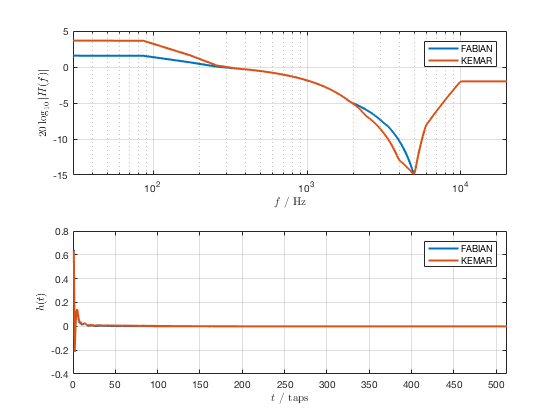
Magnitude transfer functions and impulse responses of the headphone compensation / equalization filters

Recall that there are several ways of defining which HRIR set is loaded, for example the HRIR_FILE_NAME in the SSR configuration files property, or the command line option --hrirs=FILE.

[Lindau2007]

Alexander Lindau and Stefan Weinzierl. FABIAN - Schnelle Erfassung binauraler Raumimpulsantworten in mehreren Freiheitsgraden. In Fortschritte der Akustik, DAGA Stuttgart, 2007.

[Wierstorf2011]

Hagen Wierstorf, Matthias Geier, Alexander Raake, and Sascha Spors. A Free Database of Head-Related Impulse Response Measurements in the Horizontal Plane with Multiple Distances. In 130th Convention of the Audio Engineering Society (AES), May 2011.

[SpatialAudio]

https://github.com/spatialaudio/lf-corrected-kemar-hrtfs (commit 5b5ec8)

Preparing HRIR sets¶

You can easily prepare your own HRIR sets for use with the SSR by adopting the MATLAB script data/matlab_scripts/prepare_hrirs_cipic.m to your needs. This script converts the HRIRs of the KEMAR manikin included in the CIPIC database [AlgaziCIPIC] to the format that the SSR expects. See the script for further information and how to obtain the raw HRIRs. Note that the KEMAR (CIPIC) HRIRs are not identical to the KEMAR (QU) ones.

[AlgaziCIPIC]

V. Ralph Algazi. The CIPIC HRTF database. https://www.ece.ucdavis.edu/cipic/spatial-sound/hrtf-data/.

Binaural Room Synthesis Renderer¶

Executable: ssr-brs

The Binaural Room Synthesis (BRS) renderer is a binaural renderer (refer to Section Binaural Renderer) which uses one dedicated HRIR set of each individual sound source. The motivation is to have more realistic reproduction than in simple binaural rendering. In this context HRIRs are typically referred to as binaural room impulse responses (BRIRs).

Note that the BRS renderer does not consider any specification of a virtual source’s position. The positions of the virtual sources (including their distance) are exclusively coded in the BRIRs. Consequently, the BRS renderer does not apply any distance attenuation. It only applies the respective source’s gain and the master volume. No interpolation with a Dirac as in the binaural renderer is performed for very close virtual sources. The only quantity which is explicitely considered is the orientation of the receiver, i.e. the reference. Therefore, specification of meaningful source and receiver positions is only necessary when a correct graphical illustration is desired.

The BRIRs are stored in the a format similar to the one for the HRIRs for the binaural renderer (refer to Section Binaural Renderer). However, there is a fundamental difference: In order to be consequent, the different channels do not hold the data for different positions of the virtual sound source but they hold the information for different head orientations. Explicitely,

1st channel: left ear, head orientation \(0^\circ\)
2nd channel: right ear, head orientation \(0^\circ\)
3rd channel: left ear, head orientation \(1^\circ\)
4th channel: right ear, head orientation \(1^\circ\)
…
720th channel: right ear, head orientation \(359^\circ\)

In order to assign a set of BRIRs to a given sound source an appropriate scene description in .asd-format has to be prepared (refer also to Section Audio Scenes). As shown in brs_example.asd (from the example scenes), a virtual source has the optional property properties_file which holds the location of the file containing the desired BRIR set. The location to be specified is relative to the folder of the scene file. Note that – as described above – specification of the virtual source’s position does not affect the audio processing. If you do not specify a BRIR set for each virtual source, then the renderer will complain and refuse processing the respective source.

We have measured the BRIRs of the FABIAN manikin in one of our mid-size meeting rooms called Sputnik with 8 different source positions. Due to the file size, we have not included them in the release. You can obtain the data from [BRIRs].

[BRIRs]

The Sputnik BRIRs can be obtained from here: https://dev.qu.tu-berlin.de/projects/measurements/wiki/Impulse_Response_Measurements. More BRIR repositories are compiled here: http://www.soundfieldsynthesis.org/other-resources/#impulse-responses.

Vector Base Amplitude Panning Renderer¶

Executable: ssr-vbap

The Vector Base Amplitude Panning (VBAP) renderer uses the algorithm described in [Pulkki1997]. It tries to find a loudspeaker pair between which the phantom source is located (in VBAP you speak of a phantom source rather than a virtual one). If it does find a loudspeaker pair whose angle is smaller than \(180^\circ\) then it calculates the weights \(g_l\) and \(g_r\) for the left and right loudspeaker as

\[g_{l,r} = \frac{\cos\phi \sin \phi_0 \pm \sin \phi \cos \phi_0} {2\cos \phi_0 \sin \phi_0}.\]

\(\phi_0\) is half the angle between the two loudspeakers with respect to the listening position, \(\phi\) is the angle between the position of the phantom source and the direction “between the loudspeakers”.

If the VBAP renderer can not find a loudspeaker pair whose angle is smaller than \(180^\circ\) then it uses the closest loudspeaker provided that the latter is situated within \(30^\circ\). If not, then it does not render the source. If you are in verbosity level 2 (i.e. start the SSR with the -vv option) you’ll see a notification about what’s happening.

Note that all virtual source types (i.e. point and plane sources) are rendered as phantom sources.

Contrary to WFS, non-uniform distributions of loudspeakers are ok here. Ideally, the loudspeakers should be placed on a circle around the reference position. You can optionally specify a delay for each loudspeakers in order to compensate some amount of misplacement. In the ASDF (refer to Section ASDF), each loudspeaker has the optional attribute delay which determines the delay in seconds to be applied to the respective loudspeaker. Note that the specified delay will be rounded to an integer factor of the temporal sampling period. With 44.1 kHz sampling frequency this corresponds to an accuracy of 22.676 \(\mu\)s, respectively an accuracy of 7.78 mm in terms of loudspeaker placement. Additionally, you can specify a weight for each loudspeaker in order to compensate for irregular setups. In the ASDF format (refer to Section ASDF), each loudspeaker has the optional attribute weight which determines the linear (!) weight to be applied to the respective loudspeaker. An example would be

<loudspeaker delay="0.005" weight="1.1">
        <position x="1.0" y="-2.0"/>
        <orientation azimuth="-30"/>
</loudspeaker>

Delay defaults to 0 if not specified, weight defaults to 1.

Although principally suitable, we do not recommend to use our amplitude panning algorithm for dedicated 5.1 (or comparable) mixdowns. Our VBAP renderer only uses adjacent loudspeaker pairs for panning which does not exploit all potentials of such a loudspeaker setup. For the mentioned formats specialized panning processes have been developed also employing non-adjacent loudspeaker pairs if desired.

The VBAP renderer is rather meant to be used with non-standardized setups.

[Pulkki1997]

Ville Pulkki. Virtual sound source positioning using Vector Base Amplitude Panning. In Journal of the Audio Engineering Society (JAES), Vol.45(6), June 1997.

Wave Field Synthesis Renderer¶

Executable: ssr-wfs

The Wave Field Synthesis (WFS) renderer is the only renderer so far that discriminates between virtual point sources and plane waves. It implements the simple (far-field) driving function given in [Spors2008]. Note that we have only implemented a temporary solution to reduce artifacts when virtual sound sources are moved. This topic is subject to ongoing research. We will work on that in the future. In the SSR configuration file (Section Configuration File) you can specify an overall predelay (this is necessary to render focused sources) and the overall length of the involved delay lines. Both values are given in samples.

[Spors2008]

(1, 2) Sascha Spors, Rudolf Rabenstein, and Jens Ahrens. The theory of Wave Field Synthesis revisited. In 124th Convention of the AES, Amsterdam, The Netherlands, May 17–20, 2008.

Prefiltering¶

As you might know, WFS requires a spectral correction additionally to the delay and weighting of the input signal. Since this spectral correction is equal for all loudspeakers, it needs to be performed only once on the input. We are working on an automatic generation of the required filter. Until then, we load the impulse response of the desired filter from a .wav-file which is specified via the --prefilter=FILE command line option (see Section Running SSR) or in the SSR configuration file (Section Configuration File). Make sure that the specified audio file contains only one channel. Files with a differing number of channels will not be loaded. Of course, the sampling rate of the file also has to match that of the JACK server.

Note that the filter will be zero-padded to the next highest power of 2. If the resulting filter is then shorter than the current JACK frame size, each incoming audio frame will be divided into subframes for prefiltering. That means, if you load a filter of 100 taps and JACK frame size is 1024, the filter will be padded to 128 taps and prefiltering will be done in 8 cycles. This is done in order to save processing power since typical prefilters are much shorter than typical JACK frame sizes. Zero-padding the prefilter to the JACK frame size usually produces large overhead. If the prefilter is longer than the JACK frame buffer size, the filter will be divided into partitions whose length is equal to the JACK frame buffer size.

If you do not specify a filter, then no prefiltering is performed. This results in a boost of bass frequencies in the reproduced sound field.

In order to assist you in the design of an appropriate prefilter, we have included the MATLAB script data/matlab_scripts/make_wfs_prefilter.m which does the job. In the very top of the file, you can specify the sampling frequency, the desired length of the filter as well as the lower and upper frequency limits of the spectral correction. The lower limit should be chosen such that the subwoofer of your system receives a signal which is not spectrally altered. This is due to the fact that only loudspeakers which are part of an array of loudspeakers need to be corrected. The lower limit is typically around 100 Hz. The upper limit is given by the spatial aliasing frequency. The spatial aliasing is dependent on the mutual distance of the loudspeakers, the distance of the considered listening position to the loudspeakers, and the array geometry. See [Spors2006] for detailed information on how to determine the spatial aliasing frequency of a given loudspeaker setup. The spatial aliasing frequency is typically between 1000 Hz and 2000 Hz. For a theoretical treatment of WFS in general and also the prefiltering, see [Spors2008].

The script make_wfs_prefilter.m will save the impulse response of the designed filter in a file like wfs_prefilter_120_1500_44100.wav. From the file name you can extract that the spectral correction starts at 120 Hz and goes up to 1500 Hz at a sampling frequency of 44100 Hz. Check the folder data/impules_responses/wfs_prefilters for a small selection of prefilters.

[Spors2006]

Sascha Spors and Rudolf Rabenstein. Spatial aliasing artifacts produced by linear and circular loudspeaker arrays used for Wave Field Synthesis. In 120th Convention of the AES, Paris, France, May 20–23, 2006.

Tapering¶

When the listening area is not enclosed by the loudspeaker setup, artifacts arise in the reproduced sound field due to the limited aperture. This problem of spatial truncation can be reduced by so-called tapering. Tapering is essentially an attenuation of the loudspeakers towards the ends of the setup. As a consequence, the boundaries of the aperture become smoother which reduces the artifacts. Of course, no benefit comes without a cost. In this case the cost is amplitude errors for which the human ear fortunately does not seem to be too sensitive.

In order to taper, you can assign the optional attribute weight to each loudspeaker in ASDF format (refer to Section [sec:asdf]). The weight determines the linear (!) weight to be applied to the respective loudspeaker. It defaults to 1 if it is not specified.

Ambisonics Amplitude Panning Renderer¶

Executable: ssr-aap

The Ambisonics Amplitude Panning (AAP) renderer does very simple Ambisonics rendering. It does amplitude panning by simultaneously using all loudspeakers that are not subwoofers to reproduce a virtual source (contrary to the VBAP renderer which uses only two loudspeakers at a time). Note that the loudspeakers should ideally be arranged on a circle and the reference should be the center of the circle. The renderer checks for that and applies delays and amplitude corrections to all loudspeakers that are closer to the reference than the farthest. This also includes subwoofers. If you do not want close loudspeakers to be delayed, then simply specify their location in the same direction like its actual position but at a larger distance from the reference. Then the graphical illustration will not be perfectly aligned with the real setup, but the audio processing will take place as intended. Note that the AAP renderer ignores delays assigned to an individual loudspeaker in ASDF. On the other hand, it does consider weights assigned to the loudspeakers. This allows you to compensate for irregular loudspeaker placement.

Note finally that AAP does not allow to encode the distance of a virtual sound source since it is a simple panning renderer. All sources will appear at the distance of the loudspeakers.

If you do not explicitly specify an Ambisonics order, then the maximum order which makes sense on the given loudspeaker setup will be used. The automatically chosen order will be one of \((L-1)/2\) for an odd number \(L\) of loudspeakers and accordingly for even numbers.

You can manually set the order via a command line option (Section Running SSR) or the SSR configuration file (Section Configuration File). We therefore do not explicitly discriminate between “higher order” and “lower order” Ambisonics since this is not a fundamental property. And where does “lower order” end and “higher order” start anyway?

Note that the graphical user interface will not indicate the activity of the loudspeakers since theoretically all loudspeakers contribute to the sound field of a virtual source at any time.

Conventional driving function¶

By default we use the standard Ambisonics panning function presented, for example, in [Neukom2007]. It reads

\[d(\alpha_0) = \frac{\sin\left ( \frac{2M+1}{2} \ (\alpha_0 - \alpha_\textrm{s})\right )} {(2M+1) \ \sin \left ( \frac{\alpha_0 - \alpha_\textrm{s}}{2} \right ) },\]

whereby \(\alpha_0\) is the azimuth angle of the position of the considered secondary source, \(\alpha_\textrm{s}\) is the azimuth angle of the position of the virtual source, both in radians, and \(M\) is the Ambisonics order.

In-phase driving function¶

The conventional driving function leads to both positive and negative weights for individual loudspeakers. An object (e.g. a listener) introduced into the listening area can lead to an imperfect interference of the wave fields of the individual loudspeakers and therefore to an inconsistent perception. Furthermore, conventional Ambisonics panning can lead to audible artifacts for fast source motions since it can happen that the weights of two adjacent audio frames have a different algebraic sign.

These problems can be worked around when only positive weights are applied on the input signal (in-phase rendering). This can be accomplished via the in-phase driving function given e.g. in [Neukom2007] reading

\[d(\alpha_0) = \cos^{2M} \left (\frac{\alpha_0 - \alpha_\textrm{s}}{2} \right ) \ . \nonumber\]

Note that in-phase rendering leads to a less precise localization of the virtual source and other unwanted perceptions. You can enable in-phase rendering via the according command-line option or you can set the IN_PHASE_RENDERING property in the SSR configuration file (see section Configuration File) to be TRUE or true.

[Neukom2007]

(1, 2) Martin Neukom. Ambisonic panning. In 123th Convention of the AES, New York, NY, USA, Oct. 5–8, 2007.

Distance-coded Ambisonics Renderer¶

Executable: ssr-dca

Distance-coded Ambisonics (DCA) is sometimes also termed “Nearfield Compensated Higher-Order Ambisonics”. This renderer implements the driving functions from [Spors2011]. The difference to the AAP renderer is a long story, which we will elaborate on at a later point.

Note that the DCA renderer is experimental at this stage. It currently supports orders of up to 28. There are some complications regarding how the user specifies the locations of the loudspeakers and how the renderer handles them. The rendered scene might appear mirrored or rotated. If you are experiencing this, you might want to play around with the assignment of the outputs and the loudspeakers to fix it temporarily. Or contact us.

Please bear with us. We are going to take care of this soon.

[Spors2011]

Spors, V. Kuscher, and J. Ahrens. Efficient Realization of Model-Based Rendering for 2.5-dimensional Near-Field Compensated Higher Order Ambisonics. In IEEE WASPAA, New Paltz, NY, USA, 2011.

Generic Renderer¶

Executable: ssr-generic

The generic renderer turns the SSR into a multiple-input-multiple-output convolution engine. You have to use an ASDF file in which the attribute properties_file of the individual sound source has to be set properly. That means that the indicated file has to be a multichannel file with the same number of channels like loudspeakers in the setup. The impulse response in the file at channel 1 represents the driving function for loudspeaker 1 and so on.

Be sure that you load a reproduction setup with the corresponding number of loudspeakers.

It is obviously not possible to move virtual sound sources since the loaded impulse responses are static. We use this renderer in order to test advanced methods before implementing them in real-time or to compare two different rendering methods by having one sound source in one method and another sound source in the other method.

Download the ASDF examples from http://spatialaudio.net/ssr/ and check out the file generic_renderer_example.asd which comes with all required data.

	individual delay	weight
binaural renderer	-	-
BRS renderer	-	-
VBAP renderer	+	+
WFS renderer	-	+
AAP renderer	autom.	+
generic renderer	-	-

Table 1: Loudspeaker properties considered by the different renderers.

	gain	mute	position	orientation [2]	distance attenuation	model
binaural renderer	+	+	+	+	+	only w.r.t. ampl.
BRS renderer	+	+	-	-	-	-
VBAP renderer	+	+	+	+	+	only w.r.t. ampl.
WFS renderer	+	+	+	+	+	+
AAP renderer	+	+	+	-	+	only w.r.t. ampl.
generic renderer	+	+	-	-	-	-

Table 2: Virtual source’s properties considered by the different renderers.

Summary¶

Tables 1 and 2 summarize the functionality of the SSR renderers.

[2] So far, only planar sources have a defined orientation. By default, their orientation is always pointing from their nominal position to the reference point no matter where you move them. Any other information or updates on the orientation are ignored. You can changes this behavior by using either the command line option --no-auto-rotation, using the AUTO_ROTATION configuration parameter, or hitting r in the GUI.